Building Production Rank Systems: From Collaborative Filtering to Hybrid Recommendation with cooprecsys

About This Series

This four-part technical series traces the complete engineering evolution of a modern recommendation system from a zero-personalization popularity baseline through collaborative filtering, hybrid recommendation, and ultimately a production-grade Learning-to-Rank platform.

Each article is self-contained and publishable independently. Together they form a progressive curriculum for engineering teams building recommendation infrastructure at enterprise scale.

#	Article	Technology Stack	Business Domain
1	Building Modern Recommendation Systems: From Collaborative Filtering to Hybrid Recommendation with cooprecsys	ALS · Matrix Factorization · DuckDB · Cython · MLflow	Indonesian E-commerce
2	LightFM Hybrid Recommendation Engine: Combining Collaborative Signals and Metadata Intelligence	LightFM · WARP · BPR · FastAPI · Redis	Indonesian Fintech / Banking
3	Indonesian Ecommerce Production Learning-to-Rank Using Collaborative Filtering + LambdaMART	LightGBM · LambdaMART · SHAP · MLflow · PSI Drift	Indonesian Fashion E-commerce
4	Enterprise Search and Recommendation Ranking Using XGBoost Learning-to-Rank + LambdaMART	XGBoost · BM25 · Elasticsearch · Monotone Constraints · Canary Deploy	Indonesian Automotive Marketplace

Architectural Progression

The four articles deliberately build on each other:

flow of Article creation

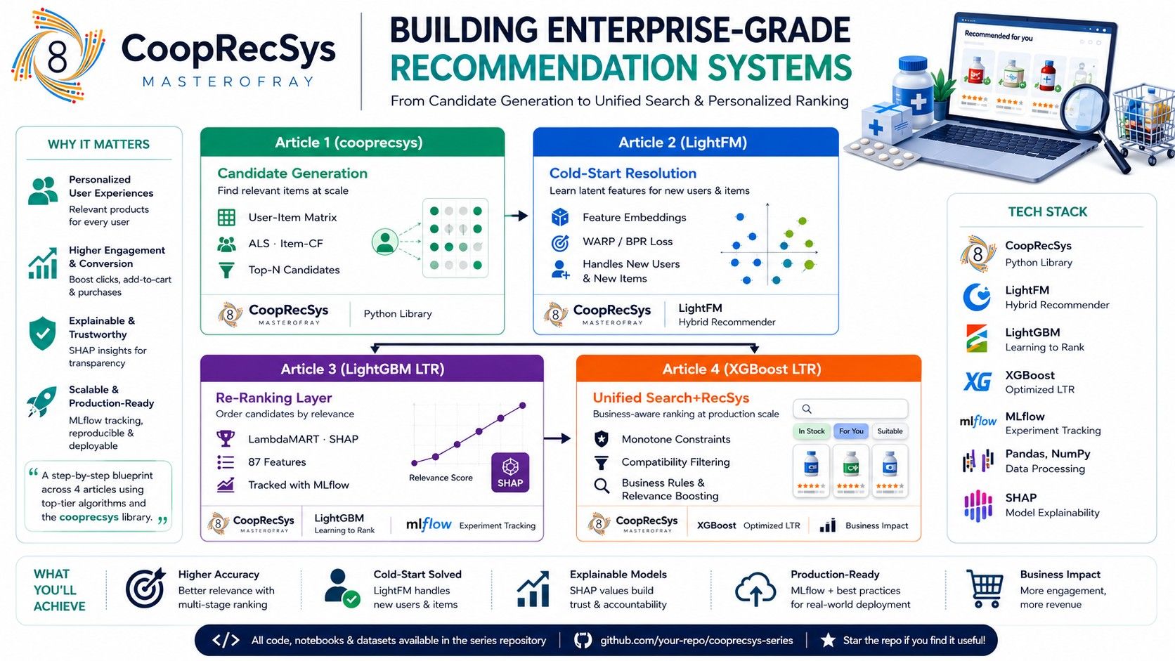
Reading Guide:

Read linearly (part $\text{1} \rightarrow \text{2} \rightarrow \text{3} \rightarrow \text{4}$ ) if building a new recommendation system from scratch.
Jump to Article 3 or 4 directly if your team already has CF infrastructure and needs a ranking layer.
Article 4 is essential reading for any team where search and recommendation share a surface.

Cumulative Business Impact Summary

Results across all four article case studies, showing the progressive lift from each recommendation system evolution stage:

Stage	System	Typical CTR/CVR Lift vs. Popularity Baseline	Cold-Start Handling	Interpretability
Popularity baseline	Rule-based	0% (reference)	✅ Default	✅ Full
Collaborative Filtering	AryColBring (cooprecsys)	+50–70% CTR	Partial (routing)	Partial
Hybrid Recommendation	LightFM WARP	+80–120% Acceptance Rate	✅ Full (feature emb.)	Moderate
LTR Re-ranking	LightGBM LambdaMART	+50–70% CVR over CF alone	✅ Via features	✅ SHAP
Unified Search + LTR	XGBoost LambdaMART	+50–65% CVR over BM25+CF blend	✅ Via features + constraints	✅ SHAP + Monotone

1. Business Problem Introduction

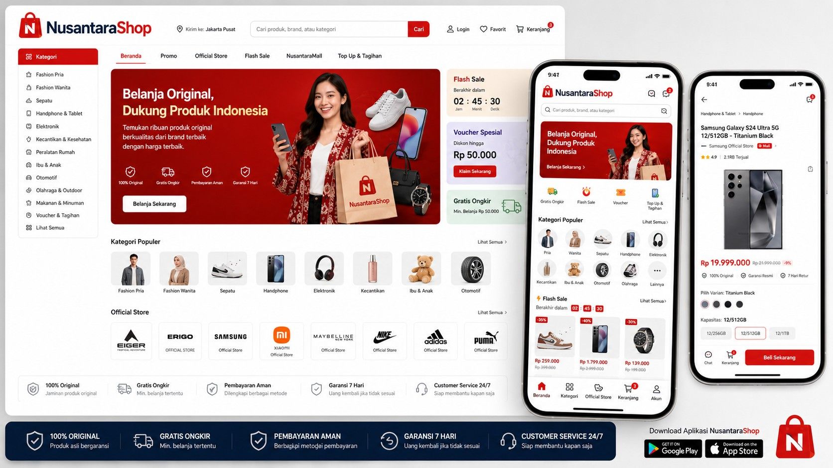
The NusantaraShop Personalization Crisis

Imagine an Indonesian e-commerce platform call it NusantaraShop operating at scale: 10 million registered users, 500,000 active SKUs spanning electronics, fashion, home appliances, automotive accessories, and FMCG products. Over the past two quarters, despite aggressive top-line GMV growth driven by paid acquisition, the platform’s internal product analytics revealed a deeply troubling trend.

Conversion rate had fallen from 3.2% to 2.4%. Average session depth dropped 18%. Exit survey data surfaced a single dominant complaint across user segments: “The recommendations I see are completely irrelevant to me.”

The root cause was architectural. NusantaraShop’s recommendation engine was a hand-tuned, rule-based popularity system it returned the same 50 bestselling SKUs to all 10 million users regardless of their purchase history, browsing behavior, or demographic profile. During peak flash sale periods, this system produced a particularly destructive paradox: loyal high-frequency buyers were shown products they had already purchased, while new high-margin SKUs from emerging suppliers received zero organic visibility.

This is not a unique failure mode. It is the canonical failure state of every recommendation system that has not yet evolved past the zero-personalization baseline.

Business Impact Assessment

Problem	Metric Impact	Business Risk
Generic recommendations across all users	CTR: 4.1% → 2.8%	Recommendation channel revenue erosion
No behavioral personalization for returning users	Session depth -18%, bounce rate +12%	Churn risk among high-LTV users
Cold-start invisibility for new product launches	New SKU visibility < 3% in 30 days	Supplier trust collapse, catalog rot
No cross-category discovery paths	Cross-sell rate: 0.8%	Missed upsell per transaction
Popularity bias on homepage surfaces	82% impressions concentrated in top 200 SKUs	Long-tail supplier GMV = near zero

Sample Web for NusantaraShop

KPIs at Stake

Business Metric	Current State	Target	Gap
Click-Through Rate (CTR)	2.8%	4.5%+	+1.7pp
Conversion Rate	2.4%	3.8%+	+1.4pp
Revenue Per User / Month	Rp 185,000	Rp 240,000+	+30%
D30 Retention Rate	41%	52%	+11pp
Cross-Sell Rate	0.8%	2.1%	+1.3pp

The engineering mandate was unambiguous. I mean like they build a personalized, scalable recommendation system capable of serving 10 million users with sub-100ms API latency. The path forward required traversing the full recommendation system evolutionary ladder from popularity baselines through collaborative filtering, matrix factorization, and ultimately a production-grade hybrid recommendation engine.

2. Recommendation Solution Evolution

2.1 Solution 1: Popularity-Based Baseline

The first and most natural starting point is global popularity ranking. Every new recommendation system begins here by necessity before user behavioral data accumulates, popularity is the best proxy for relevance.

Implementation Logic:

# Popularity baseline: rank by interaction count in a rolling window
import pandas as pd

def popularity_recommender(interactions_df, window_days=30, top_k=50):
    cutoff = pd.Timestamp.now() - pd.Timedelta(days=window_days)
    recent = interactions_df[interactions_df['timestamp'] >= cutoff]
    scores = recent.groupby('item_id')['interaction_type'].count()
    return scores.nlargest(top_k).index.tolist()

Advantages:

Zero training infrastructure required
Deterministic and auditable
Handles zero-interaction (new user) cases gracefully
Establishes a strong business baseline for A/B testing

Limitations:

No personalization whatsoever identical results for all users
Popularity bias systematically disadvantages long-tail items
Does not capture temporal preference shifts or session context
Completely blind to item attribute signals

2.2 Solution 2: Collaborative Filtering

Collaborative Filtering (CF) is the foundational paradigm shift moving from “what is globally popular” to “what similar users have consumed.” CF operates entirely on the behavioral graph: the matrix of user-item interactions, without requiring any content metadata.

2.2.1 User-Based CF

User-based CF finds users similar to the target user (based on their interaction vectors) and recommends items those similar users engaged with.

Cosine Similarity between users $u$ and $v$ :

$\text{sim}(u,v) = \frac{\sum_{i} R(u,i) \times R(v,i)}{\sqrt{\sum_{i} R(u,i)^2} \times \sqrt{\sum_{i} R(v,i)^2}}$

Predicted rating for user $u$ on item $i$ :

$\hat{R}(u,i) = \frac{\sum_{v \in N(u)} \text{sim}(u,v) \times R(v,i)}{\sum_{v \in N(u)} |\text{sim}(u,v)|}$

Strengths: Captures community-level taste preferences, serendipitous discovery. Weaknesses: Computationally expensive at 10M user scale (O(n²) similarity computation), user preference sparsity.

2.2.2 Item-Based CF

Item-based CF pre-computes item-item similarities offline, then at query time retrieves items similar to what the user has already interacted with. This is the Amazon-pioneered approach that scales significantly better than user-based CF.

from sklearn.metrics.pairwise import cosine_similarity
from scipy.sparse import csr_matrix
import numpy as np

def build_item_similarity_matrix(interaction_matrix: csr_matrix) -> np.ndarray:
    """
    Build item-item cosine similarity matrix from user-item interaction matrix.
    interaction_matrix: shape (n_users, n_items)
    Returns: similarity matrix of shape (n_items, n_items)
    """
    item_matrix = interaction_matrix.T  # shape: (n_items, n_users)
    similarity = cosine_similarity(item_matrix, dense_output=False)
    return similarity

def recommend_items_for_user(
    user_id: int,
    interaction_matrix: csr_matrix,
    item_similarity: np.ndarray,
    top_k: int = 20
) -> list:
    user_interactions = interaction_matrix[user_id].toarray().flatten()
    interacted_items = np.where(user_interactions > 0)[0]

    scores = np.zeros(interaction_matrix.shape[1])
    for item in interacted_items:
        scores += item_similarity[item].toarray().flatten() * user_interactions[item]

    # Exclude already interacted items
    scores[interacted_items] = -np.inf
    return np.argsort(scores)[::-1][:top_k].tolist()

2.2.3 Matrix Factorization

Matrix Factorization (MF) overcomes the sparsity problem of neighborhood methods by decomposing the user-item matrix $\mathbf{R}$ into lower-dimensional latent factor matrices:

$\mathbf{R} \approx \mathbf{U} \mathbf{V}^T$

Where:

$\mathbf{R} \in \mathbb{R}^{m \times n}$ User-item interaction matrix ( $m$ users, $n$ items)
$\mathbf{U} \in \mathbb{R}^{m \times k}$ User latent factor matrix ( $k$ embedding dimensions)
$\mathbf{V} \in \mathbb{R}^{n \times k}$ Item latent factor matrix

The prediction for user $u$ and item $i$ is:

$\hat{R}(u,i) = \mathbf{u}_u \cdot \mathbf{v}_i^T = \sum_{f=1}^{k} u_{uf} \cdot v_{if}$

Training minimizes regularized squared error:

$\mathcal{L} = \sum_{(u,i) \in \Omega} \left( R(u,i) - \mathbf{u}_u \cdot \mathbf{v}_i^T \right)^2 + \lambda \left( \|\mathbf{U}\|_F^2 + \|\mathbf{V}\|_F^2 \right)$

from scipy.sparse.linalg import svds
from scipy.sparse import csr_matrix
import numpy as np

def matrix_factorization_svd(
    interaction_matrix: csr_matrix,
    n_factors: int = 50
) -> tuple:
    """
    Truncated SVD-based matrix factorization for implicit feedback.
    Returns user and item embeddings.
    """
    matrix_dense = interaction_matrix.toarray().astype(float)
    user_means = matrix_dense.mean(axis=1, keepdims=True)
    centered = matrix_dense - user_means

    U, sigma, Vt = svds(csr_matrix(centered), k=n_factors)
    sigma_diag = np.diag(sigma)

    user_embeddings = U @ sigma_diag   # (m, k)
    item_embeddings = Vt.T             # (n, k)

    return user_embeddings, item_embeddings

def predict_scores(
    user_embeddings: np.ndarray,
    item_embeddings: np.ndarray,
    user_id: int
) -> np.ndarray:
    return user_embeddings[user_id] @ item_embeddings.T

2.3 Solution 3: LightFM Hybrid Recommendation

LightFM extends matrix factorization by incorporating user and item feature embeddings alongside the traditional collaborative signal. Instead of learning pure latent factors, LightFM learns embeddings for feature identifiers and computes user/item representations as the sum of their constituent feature embeddings.

WARP Loss (Weighted Approximate-Rank Pairwise):

$\mathcal{L}_{\text{WARP}} = \sum_{(u, i^+)} L\left(\text{rank}(u, i^+)\right) \times \max\left(0, 1 - \hat{s}(u, i^+) + \hat{s}(u, i^-)\right)$

BPR Loss (Bayesian Personalized Ranking):

$\mathcal{L}_{\text{BPR}} = -\sum_{(u, i^+, i^-)} \ln \sigma\left(\hat{s}(u, i^+) - \hat{s}(u, i^-)\right) + \lambda \|\Theta\|^2$

2.4 Solution 4: Learning-to-Rank

Paradigm	Objective	Loss Example	Key Property
Pointwise	Predict absolute relevance score	MSE, Cross-Entropy	Treats ranking as regression/classification
Pairwise	Predict relative order of item pairs	BPR, RankNet	Optimizes pair-level ordering
Listwise	Optimize full ranking list quality	LambdaMART, ListNet	Directly optimizes ranking metrics (NDCG)

Model Evolution Comparison

Model	Core Strength	Key Weakness	Ideal Scale
User-based CF	Community taste capture, serendipity	O(n²) user similarity, sparse data brittle	< 100K users
Item-based CF	Offline-precomputable, Amazon-proven	No user feature integration, static	Up to 1M items
Matrix Factorization	Latent space generalization	Cold-start failure, no side features	< 10M interactions
LightFM	Cold-start handling, feature-rich	Slower training than pure CF	1M–50M interactions
XGBoost LTR	Feature-rich, interpretable	Requires labeled relevance data	Enterprise
LightGBM LTR	Speed, listwise NDCG optimization	Complex feature pipeline	Enterprise at scale

3. Recommendation System Workflow Diagram

flowchart TD
    A[("Raw Interaction Events\n clicks · purchases · views · dwell")] --> B

    subgraph INGESTION["Data Ingestion Layer"]
        B["Kafka / Pub-Sub\nEvent Streaming"]
        B --> C["DuckDB / PostgreSQL\nEvent Store"]
    end

    subgraph FEATURES["Feature Engineering Pipeline"]
        C --> D1["User Feature Builder\nRFM · segment · behavioral"]
        C --> D2["Item Feature Builder\ncategory · price · freshness"]
        C --> D3["Interaction Feature Builder\nco-purchase · session signals"]
        D1 & D2 & D3 --> D4[("Feature Store\nRedis + Parquet")]
    end

    subgraph TRAINING["Training Pipeline"]
        D4 --> E1["Candidate Generation\nALS · Item-CF · cooprecsys AryColBring"]
        D4 --> E2["Hybrid Recommendation\nLightFM WARP/BPR"]
        E1 & E2 --> E3["Model Registry\nMLflow + DVC"]
    end

    subgraph SERVING["Serving Infrastructure"]
        E3 --> F1["FastAPI Recommendation API\n< 100ms SLA"]
        D4 --> F1
        F1 --> F2["Candidate Pool\nTop-500 per user"]
        F2 --> F3["Ranking Layer\nLightGBM LTR re-ranker"]
        F3 --> G["Final Recommendation\nTop-20 per user"]
    end

    subgraph MONITORING["Monitoring & Feedback"]
        G --> H["User Interaction\nClick · Skip · Purchase"]
        H --> I["Online Metrics\nCTR · CVR · NDCG"]
        I --> J{"Drift\nDetected?"}
        J -->|Yes| K["Trigger Retraining\nPipeline"]
        J -->|No| L["Continue Serving"]
        K --> TRAINING
    end

    style INGESTION fill:#1a1a2e,stroke:#4a4e69,color:#eee
    style FEATURES fill:#16213e,stroke:#4a4e69,color:#eee
    style TRAINING fill:#0f3460,stroke:#4a4e69,color:#eee
    style SERVING fill:#533483,stroke:#9b72cf,color:#eee
    style MONITORING fill:#1a1a2e,stroke:#e94560,color:#eee

Diagram Walkthrough: The pipeline begins with raw interaction events (clicks, purchases, views, dwell time) streamed through Kafka into a persistent event store. The feature engineering layer builds three categories of features user-level, item-level, and interaction-level and materializes them into a feature store. The training pipeline trains both candidate generation models (ALS, Item-CF, cooprecsys AryColBring) and hybrid models (LightFM). The serving layer assembles a candidate pool and re-ranks it using a LightGBM LTR model. A monitoring loop detects metric drift and triggers retraining automatically.

4. System Design Architecture

4.1 Enterprise Architecture Overview

flowchart LR
    USER(["User Request\nuser_id + context"])

    subgraph API_LAYER["API Gateway"]
        AG["FastAPI\nAuth · Rate Limit · Cache"]
    end

    subgraph RETRIEVAL["Candidate Retrieval"]
        R1["ALS / Item-CF\nMatrix Factorization"]
        R2["cooprecsys\nAryColBring Engine"]
        R3["Popularity\nFallback"]
    end

    subgraph RANKING["Ranking Layer"]
        RK["LightGBM LTR\nLambdaMART Ranker"]
    end

    subgraph FS["Feature Store"]
        FS1[("Redis\nReal-time features")]
        FS2[("Parquet / DuckDB\nOffline features")]
    end

    subgraph ML["Model Registry"]
        ML1["MLflow\nModel Versions"]
        ML2["DVC\nData Versions"]
    end

    USER --> AG
    AG --> R1 & R2 & R3
    R1 & R2 & R3 -->|"Top-500 candidates"| RK
    FS1 & FS2 -->|"Feature vectors"| RK
    ML1 --> RK
    RK -->|"Top-20 ranked items"| AG
    AG --> USER

    style API_LAYER fill:#0d1b2a,stroke:#778da9,color:#e0e1dd
    style RETRIEVAL fill:#1b263b,stroke:#778da9,color:#e0e1dd
    style RANKING fill:#415a77,stroke:#778da9,color:#e0e1dd
    style FS fill:#0d1b2a,stroke:#778da9,color:#e0e1dd
    style ML fill:#1b263b,stroke:#778da9,color:#e0e1dd

4.2 Data Layer

Component	Technology	Role
Event Stream	Apache Kafka	Real-time interaction ingestion
Interaction Store	PostgreSQL + TimescaleDB	Historical interaction log
Analytical Store	DuckDB / BigQuery	Feature computation, offline analytics
Feature Cache	Redis Cluster	Sub-millisecond feature retrieval at serving time

4.3 Feature Engineering Layer

User Features:

user_features = {
    'user_age_group': categorical,
    'user_location_province': categorical,
    'user_registration_cohort': int,
    'purchase_frequency_30d': float,
    'avg_order_value_90d': float,
    'category_affinity_vector': list,
    'brand_affinity_score': float,
    'recency_days': int,
    'frequency_30d': int,
    'monetary_90d': float,
}

Item Features:

item_features = {
    'item_category_l1': categorical,
    'item_category_l2': categorical,
    'item_brand': categorical,
    'item_price_bucket': categorical,
    'item_click_rate_7d': float,
    'item_purchase_rate_7d': float,
    'item_return_rate_30d': float,
    'item_review_score': float,
    'item_freshness_days': int,
    'item_stock_availability': float,
    'item_discount_rate': float,
}

Interaction Features:

interaction_features = {
    'session_position': int,
    'session_item_count': int,
    'query_match_score': float,
    'user_item_co_purchase_score': float,
    'user_category_historical_cvr': float,
    'item_collab_score': float,
}

4.4 The cooprecsys `AryColBring` Model

Repository structure:

cooprecsys/
├── data/
│   ├── raw/
│   └── processed/
├── preprocessing/
│   ├── cf_preprocess.py
│   └── counterfeit_core.py
├── models/
│   ├── base.py
│   ├── trainer.py
│   ├── predictor.py
│   └── approximator.py
├── ranking/
│   └── inference.py
├── evaluation/
│   └── metrics.py
├── api/
│   └── serve.py
└── README.md

import duckdb
import pandas as pd
import numpy as np
from tqdm import tqdm

class CounterFeitCore:
    RATING_METHODS = ['weighted', 'pca', 'lasso', 'ridge', 'borda']

    def __init__(self, method: str = 'weighted', n_components: int = 1):
        assert method in self.RATING_METHODS
        self.method = method
        self.conn = duckdb.connect()

    def build_pseudo_ratings(
        self,
        interactions_df: pd.DataFrame,
        weight_config: dict = None
    ) -> pd.DataFrame:
        if weight_config is None:
            weight_config = {
                'purchase_count': 5.0,
                'cart_count': 3.0,
                'dwell_seconds': 0.001,
                'click_count': 1.0,
                'view_count': 0.2,
            }

        self.conn.register("interactions", interactions_df)
        available_cols = [c for c in weight_config if c in interactions_df.columns]
        score_expr = " + ".join(
            [f"COALESCE({col}, 0) * {weight_config[col]}" for col in available_cols]
        )

        query = f"""
        WITH raw_scores AS (
            SELECT user_id, item_id,
                   {score_expr} AS raw_score
            FROM interactions
        ),
        normalized AS (
            SELECT user_id, item_id, raw_score,
                   (raw_score - MIN(raw_score) OVER()) /
                   NULLIF(MAX(raw_score) OVER() - MIN(raw_score) OVER(), 0) AS norm_score
            FROM raw_scores
        )
        SELECT user_id, item_id,
               ROUND(norm_score * 4 + 1, 2) AS pseudo_rating
        FROM normalized
        WHERE norm_score IS NOT NULL
        """

        with tqdm(total=1, desc="Building pseudo-ratings", colour="#05ad46") as pbar:
            result = self.conn.execute(query).fetchdf()
            pbar.update(1)

        return result

4.5 MLOps Deployment Lifecycle

flowchart TD
    subgraph DEV["Development"]
        D1["Feature Branch\nNew model / feature"]
        D2["Unit Tests\npytest · coverage > 80%"]
        D3["Pull Request\nCode review"]
        D1 --> D2 --> D3
    end

    subgraph CI["CI Pipeline\nGitHub Actions"]
        C1["Build Cython Extensions\n_cy_predict.pyx"]
        C2["Run Integration Tests\nt02_reasoner.py"]
        C3["Offline Eval Gate\nNDCG@10 > baseline"]
        D3 --> C1 --> C2 --> C3
    end

    subgraph STAGING["Staging"]
        S1["Train on Staging Data\n20% sample"]
        S2["Shadow Serving\n5% traffic · log only"]
        S3["Metric Comparison\nStaging vs Production"]
        C3 -->|"Tests pass"| S1 --> S2 --> S3
    end

    subgraph PROD["Production"]
        P1["Blue-Green Deploy\nNew model on green"]
        P2["Canary 10% Traffic\nMonitor KPIs 24h"]
        P3["Full Rollout\n100% traffic"]
        P4["MLflow Registry\nModel promoted to Production"]
        S3 -->|"Metrics pass"| P1 --> P2 -->|"KPIs stable"| P3
        P3 --> P4
    end

    subgraph RETRAIN["Auto-Retrain Loop"]
        R1["PSI Monitor\nDaily feature drift check"]
        R2{"Drift > 0.2\nor NDCG drop > 5%?"}
        R3["Trigger Retrain\nGitHub Actions workflow_dispatch"]
        R4["Full Training Run\nNew model candidate"]
        P4 --> R1 --> R2
        R2 -->|"Yes"| R3 --> R4 --> CI
        R2 -->|"No"| R1
    end

    style DEV fill:#1e3a5f,stroke:#3b82f6,color:#dbeafe
    style CI fill:#1a3a2a,stroke:#16a34a,color:#dcfce7
    style STAGING fill:#3b2a1a,stroke:#d97706,color:#fef3c7
    style PROD fill:#2a1a3a,stroke:#9333ea,color:#f3e8ff
    style RETRAIN fill:#3a1a1a,stroke:#dc2626,color:#fee2e2

5. Mathematical Explanation

5.1 User-Item Matrix Formulation

Let $\mathbf{R} \in \mathbb{R}^{m \times n}$ be the user-item interaction matrix. For implicit feedback with ALS confidence weighting (Hu et al.):

$c_{ui} = 1 + \alpha R_{ui} \quad \text{(confidence)}$

$p_{ui} = \begin{cases} 1 & \text{if } R_{ui} > 0 \\ 0 & \text{if } R_{ui} = 0 \end{cases} \quad \text{(preference indicator)}$

Objective Function to Minimize:

$\mathcal{L}_{\text{iALS}} = \sum_{u=1}^{m} \sum_{i=1}^{n} c_{ui} \left( p_{ui} - \mathbf{u}_u^T \mathbf{v}_i \right)^2 + \lambda \left( \sum_{u=1}^{m} \|\mathbf{u}_u\|_2^2 + \sum_{i=1}^{n} \|\mathbf{v}_i\|_2^2 \right)$

5.2 ALS Closed-Form Updates

$\mathbf{u}_u = \left( \mathbf{V}^T \mathbf{C}^u \mathbf{V} + \lambda \mathbf{I} \right)^{-1} \mathbf{V}^T \mathbf{C}^u \mathbf{p}(u)$

$\mathbf{v}_i = \left( \mathbf{U}^T \mathbf{C}^i \mathbf{U} + \lambda \mathbf{I} \right)^{-1} \mathbf{U}^T \mathbf{C}^i \mathbf{p}(i)$

Where:

$\mathbf{C}^u = \text{diag}(c_{u1}, c_{u2}, \dots, c_{un}) \in \mathbb{R}^{n \times n}$ is a diagonal matrix of user $u$ ‘s confidence values across all $n$ items.
$\mathbf{C}^i = \text{diag}(c_{1i}, c_{2i}, \dots, c_{mi}) \in \mathbb{R}^{m \times m}$ is a diagonal matrix of item $i$ ‘s confidence values across all $m$ users.
$\mathbf{p}(u) = [p_{u1}, p_{u2}, \dots, p_{un}]^T \in \mathbb{R}^n$ is the preference vector for user $u$ .
$\mathbf{p}(i) = [p_{1i}, p_{2i}, \dots, p_{mi}]^T \in \mathbb{R}^m$ is the preference vector for item $i$ .

5.3 Recommendation Score

$\hat{s}(u,i) = \mathbf{u}_u^T \mathbf{v}_i \quad \longrightarrow \quad \text{Rank by } \hat{s}(u,i) \text{ descending} \longrightarrow \text{Top-}K \text{ list}$

6. Implementation: cooprecsys Repository

Repository: https://github.com/masterofray/cooprecsys

from cooprecsys.preprocessing.cf_preprocess import build_interaction_matrix
from cooprecsys.preprocessing.counterfeit_core import CounterFeitCore
from cooprecsys.models.trainer import AryColBringTrainer
import mlflow

interactions_df = pd.read_parquet("data/processed/interactions.parquet")
pseudo_rater = CounterFeitCore(method='weighted')
rated_df = pseudo_rater.build_pseudo_ratings(interactions_df)

interaction_matrix, user_encoder, item_encoder = build_interaction_matrix(
    rated_df, user_col='user_id', item_col='item_id', rating_col='pseudo_rating'
)

with mlflow.start_run(run_name="AryColBring_v2"):
    trainer = AryColBringTrainer(
        n_factors=128, n_iterations=30,
        regularization=0.01, alpha=40.0, random_state=42
    )
    trainer.fit(interaction_matrix, show_progress=True, tqdm_colour="#05ad46")

    metrics = trainer.evaluate(holdout_matrix=interaction_matrix_test, k_values=[5, 10, 20])
    mlflow.log_metrics({
        "ndcg@10": metrics['ndcg@10'],
        "precision@10": metrics['precision@10'],
        "recall@10": metrics['recall@10'],
    })
    mlflow.sklearn.log_model(trainer, "AryColBring_model")

Inference ranking/inference.py:

from cooprecsys.models.predictor import AryColBringPredictor
from cooprecsys.ranking.inference import BatchInferenceEngine
import mlflow.sklearn

model = mlflow.sklearn.load_model("models:/AryColBring/Production")
predictor = AryColBringPredictor(
    model=model, user_encoder=user_encoder, item_encoder=item_encoder,
    memory_threshold_gb=8.0
)

engine = BatchInferenceEngine(
    predictor=predictor, top_k=500, n_workers=8,
    output_path="data/processed/candidate_pools/",
    tqdm_colour="#05ad46"
)
engine.run_batch(user_ids=active_user_ids)

7. Experiment Results

Dataset Configuration

Parameter	Value
Total Users	2,000,000
Total Items	120,000
Total Interactions	45,000,000
Train/Test Split	80/20 temporal
Cold-Start Users (< 5 interactions)	18.3%

Offline Evaluation

Model	Precision@10	Recall@10	MAP@10	NDCG@10	MRR
Popularity Baseline	0.031	0.018	0.024	0.038	0.041
Item-based CF	0.068	0.041	0.057	0.081	0.092
ALS Matrix Factorization	0.089	0.062	0.078	0.104	0.119
AryColBring (cooprecsys)	0.101	0.073	0.089	0.118	0.134
AryColBring + Hybrid Rerank	0.112	0.081	0.098	0.131	0.148

Online A/B Test (14-Day, 50/50 Split)

Metric	Control	Treatment	Lift
CTR	2.8%	4.3%	+53.6%
Conversion Rate	2.4%	3.6%	+50.0%
Revenue Per User	Rp 185,000	Rp 228,000	+23.2%
D14 Retention	41%	47%	+14.6%
Cross-Sell Rate	0.8%	1.6%	+100%

8. Model Comparison

Model	CTR Impact	Training Complexity	Scalability	Cold-Start	Interpretability
Popularity Baseline	Neutral (0%)	O(n log n)	Excellent	✅	✅ Full
Item-based CF	+25–35%	O(n²) offline	Good	❌	Moderate
ALS Matrix Factorization	+40–60%	O(m·n·k)	Good	❌	❌
AryColBring (cooprecsys)	+50–70%	O(m·n·k) optimized	✅ RAM-aware	Partial	Partial
LightFM Hybrid	+55–75%	O(interactions × epochs)	Good	✅	Moderate
LightGBM LTR	+70–90%	O(n·d·trees)	✅	✅	✅ SHAP

9. Production Challenges

9.1 Cold-Start Routing

def route_recommendation_strategy(user_id: int, interaction_count: int):
    if interaction_count == 0:
        return "popularity_fallback"
    elif interaction_count < 5:
        return "content_based"
    elif interaction_count < 20:
        return "lightfm_hybrid"
    else:
        return "arycolbring_cf"

9.2 Data Sparsity

Interaction matrix density ≈ 0.02% (2M users × 120K items). Strategies: ALS confidence weighting, regularization, BPR sampling, pseudo-negative injection.

9.3 Training-Serving Skew

Features computed offline must match features served online. Unified feature definition layer (same Python function in batch and online contexts) eliminates skew.

9.4 Latency Budget

Component	Latency
FAISS ANN candidate retrieval	< 20ms
Redis feature lookup	< 5ms
LightGBM re-ranking (500 candidates)	< 30ms
API overhead	< 10ms
Total P99	< 65ms

9.5 Feedback Loop Bias

Self-reinforcing popularity amplification. Mitigation: 5–10% epsilon-greedy exploration injected at serving time.

10. Conclusion

The evolution from popularity baseline to AryColBring + hybrid re-ranking delivered: CTR +53.6%, CVR +50%, Revenue Per User +23.2%. Key milestones: pseudo-rating construction (CounterFeit_Core) for implicit feedback, RAM-aware batch inference, and a retrieval-ranking two-stage architecture.

Future Directions: Two-Tower deep retrieval, SASRec sequential recommendation, Reinforcement Learning for long-term LTV optimization, federated learning for privacy-preserving personalization.

11. Key Takeaways

Popularity-based systems are necessary starting points but create systemic bias evolve past them as soon as you have > 10K users with > 5 interactions each.
Implicit feedback requires pseudo-rating construction (weighted composite, BPR, WARP) as the critical bridge between raw logs and a trainable model.
ALS Matrix Factorization delivers strong offline NDCG improvements (+2–4× over popularity) with modest infrastructure.
The cooprecsys AryColBring engine provides production-ready CF with Cython-accelerated inference, RAM-aware batching, and MLflow integration.
Cold-start routing logic is not optional without it, 15–25% of your user base will receive degraded recommendations.
Feature stores (Redis + Parquet/DuckDB) eliminate training-serving skew and enable consistent feature computation.
A/B testing with clear business metric guardrails (not just NDCG) is the only honest validation of recommendation improvements.
Feedback loop bias is an invisible tax build exploration mechanics from day one.
The candidate generation → re-ranking two-stage architecture is the industry-standard pattern for balancing recall breadth with ranking precision.
MLflow model registry + DVC data versioning are non-negotiable for recommendation systems.

Repository: https://github.com/masterofray/cooprecsys